How can humans or machines interact with an environment and learn a strategy for selecting actions that are beneficial to their goals? Answers to this question fall under the artificial intelligence category of reinforcement learning. Here I am going to provide an introduction to temporal difference (TD) learning, which is the algorithm at the heart of reinforcement learning.
I will be presenting TD learning from a computational neuroscience background. My post has been heavily influenced by Dayan and Abbott Ch 9, but I have added some additional points. The ultimate reference for reinforcement learning is the book by Sutton and Barto, and their chapter 6 dives into TD learning.
Conditioning
To start, let’s review conditioning. The most famous example of conditional is Pavlov’s dogs. The dogs naturally learned to salivate upon the delivery of food, but Pavlov realized that he could condition dogs to associate the ringing of a bell with the delivery of food. Eventually, the ringing of the bell on its own was enough to cause dogs to salivate.
The specific example of Pavlov’s dogs is an example of classical conditioning. In classical conditioning, no action needs to be taken. However, animals can also learn to associate actions with rewards and this is called operant conditioning.
Before I introduce some specific conditioning paradigms, here are the important definitions:
 = stimulus
 = reward
 = no reward
 = value, or expected reward (generally a function of , )
 = binary, indicator variable, of stimulus (1 if stimulus present, 0 otherwise)
Here are the conditioning paradigms I want to discuss:
- Pavlovian
- Extinction
- Blocking
- Inhibitory
- Secondary
For each of these paradigms, I will introduce the necessary training stages and the final result. The statement,  , means that
  becomes associated (
 ) with
  .
.
Pavlovian
Training:  . The stimulus is trained with a reward.
Results: ![s \rightarrow v[r]](https://s0.wp.com/latex.php?latex=s+%5Crightarrow+v%5Br%5D&bg=ffffff&fg=444444&s=0&c=20201002) . The stimulus is associated with the expectation of a reward.
. The stimulus is associated with the expectation of a reward.
Extinction
Training 1: . The stimulus is trained with a reward. This eventually leads to successful Pavlovian training.
Training 2:  . The stimulus is trained with a no reward.
Results: ![s \rightarrow v[x]](https://s0.wp.com/latex.php?latex=s+%5Crightarrow+v%5Bx%5D&bg=ffffff&fg=444444&s=0&c=20201002) . The stimulus is associated with the expectation of no reward. Extinction of the previous Pavlovian training.
. The stimulus is associated with the expectation of no reward. Extinction of the previous Pavlovian training.
Blocking
Training 1:  . The first stimulus is trained with a reward. This eventually leads to successful Pavlovian training.
Training 2:  . The first stimulus and a second stimulus is trained with a reward.
Results: ![s_1 \rightarrow v[r]](https://s0.wp.com/latex.php?latex=s_1+%5Crightarrow+v%5Br%5D&bg=ffffff&fg=444444&s=0&c=20201002) , and
, and ![s_2 \rightarrow v[x]](https://s0.wp.com/latex.php?latex=s_2+%5Crightarrow+v%5Bx%5D&bg=ffffff&fg=444444&s=0&c=20201002) . The first stimulus completely explains the reward and hence “blocks” the second stimulus from being associated with the reward.
. The first stimulus completely explains the reward and hence “blocks” the second stimulus from being associated with the reward.
Inhibitory
Training:  , and . The combination of two stimuli leads to no reward, but the first stimuli is trained with a reward.
Results: , and ![s_2 \rightarrow -v[r]](https://s0.wp.com/latex.php?latex=s_2+%5Crightarrow+-v%5Br%5D&bg=ffffff&fg=444444&s=0&c=20201002) . The first stimuli is associated with the expectation of the reward while the second stimuli is associated with the negative of the reward.
. The first stimuli is associated with the expectation of the reward while the second stimuli is associated with the negative of the reward.
Secondary
Training 1: . The first stimulus is trained with a reward. This eventually leads to successful Pavlovian training.
Training 2:  . The second stimulus is trained with the first stimulus.
Results: ![s_2 \rightarrow v[r]](https://s0.wp.com/latex.php?latex=s_2+%5Crightarrow+v%5Br%5D&bg=ffffff&fg=444444&s=0&c=20201002) . Eventually the second stimulus is associated with the reward despite never being directly associated with the reward.
. Eventually the second stimulus is associated with the reward despite never being directly associated with the reward.
Rescorla-Wagner Rule
How do we turn the various conditioning paradigms into a mathematical framework of learning? The Rescorla Wagner rule (RW) is a very simple model that can explain many, but not all, of the above paradigms.
The RW rule is a linear prediction model that requires these three equations:


and introduces the following new terms:
 = weights associated with stimuli state
 = learning rate, with
What do each of these equations actually mean?
- The expected reward, , is a linear dot product of a vector of weights, , associated with each stimuli, .
- But there may be a mismatch, or error, between the true actual reward, , and the expected reward, .
- Therefore we should update our weights of each stimuli. We do this by adding a term that is proportional to a learning rate , the error
 , and the stimuli .
During a Pavlovian pairing of stimuli with reward, the RW rule predicts an exponential approach of the weight to  over the course of several trials for most values of (if
  it would instantly update to the final value. Why is this usually bad?). Then if the reward stops being paired with the stimuli, the weight will exponential decay over the course of the next trials.
The RW rule will also continue to work when the reward/stimulus pairing is stochastic instead of deterministic and the will will still approach the final value of .
How does blocking fit into this framework? Well the RW rule says that after the first stage of training, the weights are  and
and  (since we have not presented stimulus two). When we start the second stage of training and try and associate stimulus two with the reward, we find that we cannot learn that association. The reason is that there is no error (hence
  ) and therefore forever. If instead we had only imperfectly learned the weight of the first stimulus, then there is still some error and hence some learning is possible.
One thing that the RW rule incorrectly predicts is secondary conditioning. In this case, during the learning of the first stimulus,  , the learned weight becomes
  . The RW rule predicts that the second stimulus,
  , will become
  . This is because this paradigm is exactly the same as inhibitory conditioning, according to the RW rule. Therefore, a more complicated rule is required to successfully have secondary conditioning
One final note. The RW rule can provide an even better match to biology by assuming a non-linear relationship between and the animal behavior. This function is often something that exponentially saturates at the maximal reward (ie an animal is much more motivated to go from 10% to 20% of the max reward rather than from 80% to 90% of the max reward). While this provides a better fit to many biological experiments, it still cannot explain the secondary conditioning paradigm.
Temporal Difference Learning
To properly model secondary conditioning, we need to explicitly add in time to our equations. For ease, one can assume that time,  , is discrete and that a trial lasts for total time
  and therefore
  .
.
The straightforward (but wrong) extension of the RW rule to time is:
![v[t]=w[t-1] \cdot u[t]](https://s0.wp.com/latex.php?latex=v%5Bt%5D%3Dw%5Bt-1%5D+%5Ccdot+u%5Bt%5D&bg=ffffff&fg=444444&s=0&c=20201002)
![\delta[t] = r[t]-v[t]](https://s0.wp.com/latex.php?latex=%5Cdelta%5Bt%5D+%3D+r%5Bt%5D-v%5Bt%5D&bg=ffffff&fg=444444&s=0&c=20201002)
![w[t] = w[t-1]+\epsilon \delta[t] u[t]](https://s0.wp.com/latex.php?latex=w%5Bt%5D+%3D%C2%A0w%5Bt-1%5D%2B%5Cepsilon+%5Cdelta%5Bt%5D+u%5Bt%5D&bg=ffffff&fg=444444&s=0&c=20201002)
where we will say that it takes one time unit to update the weights.
Why is this naive RW with time wrong? Well, psychology and biology experiments show that animals expected rewards does NOT reflect the past history of rewards nor just reflect the next time step, but instead reflects the expected rewards during the WHOLE REMAINDER of the trial. Therefore a better match to biology is:
![R[t]= \langle \sum_{\tau=0}^{T-t} r[t+\tau] \rangle](https://s0.wp.com/latex.php?latex=R%5Bt%5D%3D+%5Clangle+%5Csum_%7B%5Ctau%3D0%7D%5E%7BT-t%7D+r%5Bt%2B%5Ctau%5D+%5Crangle&bg=ffffff&fg=444444&s=0&c=20201002)
![\delta[t] = R[t]-v[t]](https://s0.wp.com/latex.php?latex=%5Cdelta%5Bt%5D+%3D+R%5Bt%5D-v%5Bt%5D&bg=ffffff&fg=444444&s=0&c=20201002)
where ![R[t]](https://s0.wp.com/latex.php?latex=R%5Bt%5D&bg=ffffff&fg=444444&s=0&c=20201002) is the full reward expected over the remainder of the trial while
is the full reward expected over the remainder of the trial while ![r[t]](https://s0.wp.com/latex.php?latex=r%5Bt%5D&bg=ffffff&fg=444444&s=0&c=20201002) remains the reward at a single time step. This is closer to biology, but we are still missing a key component. Not all future rewards are treated equally. Instead, rewards that happen sooner are valued higher than rewards in the distant future (this is called discounting). So the best match to biology is the following:
remains the reward at a single time step. This is closer to biology, but we are still missing a key component. Not all future rewards are treated equally. Instead, rewards that happen sooner are valued higher than rewards in the distant future (this is called discounting). So the best match to biology is the following:
![R[t]= \langle \sum_{\tau=0}^{T-t} \gamma^\tau r[t+\tau] \rangle](https://s0.wp.com/latex.php?latex=R%5Bt%5D%3D+%5Clangle+%5Csum_%7B%5Ctau%3D0%7D%5E%7BT-t%7D+%5Cgamma%5E%5Ctau+r%5Bt%2B%5Ctau%5D+%5Crangle&bg=ffffff&fg=444444&s=0&c=20201002)
where  is the discounting factor for future rewards. A small discounting factor implies we prefer rewards now while a large discounting factor means we are patient for our rewards.
We have managed to write down a set of equations that accurately summarize biological reinforcement. But how can we actually learn with this system? As currently written, we would need to know the average reward over the remainder of the whole trial. Temporal difference learning makes the following assumptions in order to solve for the expected future rewards:
- Future rewards are Markovian
- Current observed estimate of reward is close enough to the typical trial
A Markov process is memoryless in that the next future step only depends on the current state of the system and has no other history dependence. By assuming rewards follow this structure, we can make the following approximation:
The second approximation is called bootstrapping. We will use the currently observed values rather than the full estimate for future rewards. So finally we end up at the temporal difference learning equations:
![R[t] = r[t+1] + \gamma v[t+1]](https://s0.wp.com/latex.php?latex=R%5Bt%5D+%3D+%C2%A0r%5Bt%2B1%5D+%2B+%5Cgamma+v%5Bt%2B1%5D&bg=ffffff&fg=444444&s=0&c=20201002)
![\delta[t] =r[t+1] + \gamma v[t+1]-v[t]](https://s0.wp.com/latex.php?latex=%5Cdelta%5Bt%5D+%3Dr%5Bt%2B1%5D+%2B+%5Cgamma+v%5Bt%2B1%5D-v%5Bt%5D&bg=ffffff&fg=444444&s=0&c=20201002)
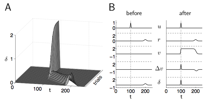
Dayan and Abbott, Figure 9.2. This illustrates TD learning in action.
I have included an image from Dayan and Abbott about how TD learning evolves over consecutive trials, please read their Chapter 9 for full details.
Finally, I should mention that in practice, people often use the TD-Lambda algorithm. This version introduces a new parameter, lambda, which controls how far back in time one can make adjustments. Lambda 0 implies one time step only, while lambda 1 implies all past time steps. This allows TD learning to excel even if the full system is not Markovian.
Dopamine and Biology’s TD system
So does biology actually implement TD learning? Animals definitely utilize reinforcement learning and there is strong evidence that temporal difference learning plays an essential role. The leading contender for the reward signal is dopamine. This is a widely used neurotransmitter that evolved in early animals and remains widely conserved. There are a relatively small number of dopamine neurons (in the basal ganglia and VTA in humans) that project widely throughout the brain. These dopamine neurons can produce an intense sensation of pleasure (and in fact the “high” of drugs often comes about either through stimulating dopamine production or preventing its reuptake).
There are two great computational neuroscience papers that highlight the important connection between TD learning and dopamine that analyze two different biological systems:
Both of these papers deserved to be read in detail, but I’ll give a brief summary of the bee foraging paper here. Experiments were done that tracked bees in an controlled environment consisting of “yellow flowers” and “blue flowers” (which were basically just different colored cups). These flowers had the same amount of nectar on average, but were either consistent or highly variable. The bees quickly learned to only target the consistent flowers. These experimental results were very well modeled by assuming the bee was performing TD learning with a relatively small discount factor (driving it to value recent rewards).
TD Learning and Games
Playing games is the perfect test bed for TD learning. A game has a final objective (win), but throughout play it can be difficult to determine your probability of winning. TD learning provides a systematic framework to associate the value of a given game state with the eventual probability of learning. Below I highlight the games that have most significantly showcased the usefulness of reinforcement learning.
Backgammon
Backgammon is a two person game of perfect information (neither player has hidden knowledge) with an element of chance (rolling dice to determine one’s possible moves). Gerald Tesauro’s TD-Gammon was the first program to showcase the value of TD learning, so I will go through it in more detail.
Before getting into specifics, I need to point out that there are actually two (often competing) branches in artificial intelligence:
Symbolic logic tends to be a set of formal rules that a system needs to follow. These rules need to be designed by humans. The connectionist approach uses artificial neural networks and other approaches like TD learning that attempt to mimic biological neural networks. The idea is that humans set up the overall architecture and model of the neural network, but the specific connections between “neurons” is determined by the learning algorithm as it is fed real data examples.
Tesauro actually created two versions of a backgammon program. The first was called Neurogammon. It was trained using supervised learning where it was given expert games as well as games Tesauro played against himself and told to learn to mimic the human moves. Neurogammon was able to play at an intermediate human level.
Tesauro’s next version of a backgammon program was TD-Gammon since it used the TD learning rule. Instead of trying to mimic the human moves, TD-Gammon used to the TD learning rule to assign a score to each move throughout a game. The additional innovation is that the TD-Gammon program was trained by playing games against itself. This initial version of TD-Gammon soon matched Neurogammon (ie intermediate human level). TD-Gammon was able to beat experts by both using a supervised phase on expert games as well as a reinforcement phase.
Despite being able to beat experts, TD-Gammon still had a weakness in the endgame. Since it only looked two-moves ahead, it could miss key moves that would have been found by a more thorough analytical approach. This is where symbolic logic excels and hence TD-Gammon was a great demonstration of the complimentary strength and weaknesses of symbolic vs connectionist logic.
Go
Go is a two person game of perfect information with no element of chance. Despite this perfect knowledge, the game is complex enough that there are around  possible games (for reference, there are only about
  atoms in the whole universe). So despite the perfect information, there are just too many possible games to determine the optimal move.
Recently AlphaGo made a huge splash by beating one of the world’s top players of Go. Most Go players, and even many artificial intelligence researchers, thoughts an expert level Go program was years away. So the win was just as surprising as when DeepBlue beat Kasparov in chess. AlphaGo is a large program with many different parts, but at the heart of it is a reinforcement learning module that utilizes TD learning (see here or here for details).
Poker
The final frontier in gaming is poker, specifically multi-person No-Limit Texas Hold’em. The reason this is the toughest game left is that it is a multi-player game with imperfect information and an element of chance.
Last winter the computer systems won against professionals for the first time in a series of heads up matches (computer vs only one human). Further improvements are needed to actually beat the best professionals at a multi-person table, but these results seem encouraging for future successes. The interesting thing to me is that both AI system seems to have used only a limited amount of reinforcement learning. I think that fully embracing reinforcement and TD learning should be the top priority for these research teams and might provide the necessary leap in ability. And they should hurry since others might beat them to it!


![R[t]= \langle r[t+1] \rangle + \gamma \langle \sum_{\tau=1}^{T-t} \gamma^{\tau-1} r[t+\tau]](https://s0.wp.com/latex.php?latex=R%5Bt%5D%3D+%5Clangle+r%5Bt%2B1%5D+%5Crangle+%2B+%5Cgamma+%5Clangle+%5Csum_%7B%5Ctau%3D1%7D%5E%7BT-t%7D+%5Cgamma%5E%7B%5Ctau-1%7D+r%5Bt%2B%5Ctau%5D&bg=ffffff&fg=444444&s=0&c=20201002)
![R[t]= \langle r[t+1] \rangle + \gamma R[t+1]](https://s0.wp.com/latex.php?latex=R%5Bt%5D%3D+%5Clangle+r%5Bt%2B1%5D+%5Crangle+%2B+%5Cgamma+R%5Bt%2B1%5D&bg=ffffff&fg=444444&s=0&c=20201002)
 neuron. I will define a neuron’s state as
  and neuron
  (out of
  total) is firing if
  and not firing if
  .
. of them) that one wants to store as
  where
where  . The idea is to define the interactions between neurons as:

 ) by examining the activation function of the first neuron.


 . Second, we will assume that memories are not biased (equal numbers of neurons are on and off). Third, we will assume that we are storing random memories. Then using the central limit theorem, we get that on average,
  . (Advanced question: what is the standard deviation of the noise term? What does that imply about stability of memories?)
 ). Using similar arguments as above, one can show that on average each memory has an energy of
  and that a flipping a single spin leads to higher energy. (Fundamental question: prove these statements!)
 , and create a dynamical system with these memories as global minima.
 are hidden neurons (if present, not a requirement). There are three different types of interactions, those amongst visible neurons only (
 ), those amongst hidden neurons only (
 ), and those between visible and hidden neurons (
 and/or correlated with each other?
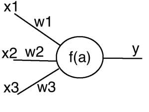

 , to determine the output,
  . There are lots of different possible activation rules with some popular ones including


 , where each entry
  is
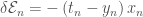
is  . Then training proceeds by seeing if the output label of a perceptron matches the correct label. If everything is correct, perfect! If not, we need to do something with that error.
![\mathcal{E} = - \sum_n \left[ t_n \ln y_n + \left(1-t_n \right) \ln \left(1-y_n \right) \right]](https://s0.wp.com/latex.php?latex=%5Cmathcal%7BE%7D+%3D+-+%5Csum_n+%5Cleft%5B+t_n+%5Cln+y_n+%2B+%5Cleft%281-t_n+%5Cright%29+%5Cln+%5Cleft%281-y_n+%5Cright%29+%5Cright%5D+&bg=ffffff&fg=444444&s=0&c=20201002)
 .
. . This is a greedy algorithm (always improves current error, longterm consequences be damned!). Gradient descent comes in several closely related varieties: online, batch, and mini-batch. Let’s start with the mini-batch. First the data is divided up into small random sets (say 10 data points each). Then we loop through the mini-batches, and for each one we calculate the output and error and update the weights. Online learning is when the mini-batches each contain exactly 1 data point, while batch learning is when the mini-batch is the whole dataset. The current standard is to use a mini-batch of between 10 to 100 which is a compromise between speed (batches are faster) and accuracy (online finds better solutions).