Deep Learning Seminar Course

This semester Terry Sejnowski is teaching a graduate seminar course that is focused on Deep Learning. The course meets weekly for two hours to discuss papers. Here I’ll just outline the course and in later posts I’ll add some thoughts on each specific week.

Week 1: Perceptrons

Week 2: Hopfield Nets and Boltzmann Machines

Week 3: Backprop

Week 4: Independent Component Analysis (ICA)

Week 5: Convolutional Neural Networks (CNN)

Week 6: Recurrent Neural Networks (RNN)

Week 7: Reinforcement Learning

Week 8: Information and Control Theory

Advertisement

I3: International Institute for Intelligence

While I was previously discussing my opinion of Open AI, I mentioned that I would do something different if I was in charge. Here is my dream.


What OpenAI is Missing

Helping everyday people throughout the whole world.

OpenAI’s stated goal is:

OpenAI is a non-profit artificial intelligence research company. Our goal is to advance digital intelligence in the way that is most likely to benefit humanity as a whole, unconstrained by a need to generate financial return.

In the short term, we’re building on recent advances in AI research and working towards the next set of breakthroughs.

However, based on their actions so far, this interview with Ilya Sutskever, and popular press articles, the main focus of OpenAI appears to be advanced research in an artificial intelligence by stressing open source, as well as thinking longterm about the impacts of letting advanced artificial intelligence systems control large aspects of our life. While I strongly support these goals, in reality, these will not benefit all of humanity. Instead, it only benefits those with either the necessary training (which is a minimum of a bachelors, but usually means a masters or PhD) or money (to hire top people, buy the required computing resources, etc) to take advantage of the advanced research. So this leaves out the developing world as well as the poor in developed countries, ie contrary to their stated goal, OpenAI is missing the vast majority of humanity.

While one can argue that by making OpenAI’s research open source, eventually it will trickle down and help a wider swath of humanity. However, the current trend suggests that large corporations are best poised to benefit the most from the next revolution (I mean, who is more likely to invent a self driving car, Google, or someone in a developing country?). Additionally, these innovations focus on first world problems (since these are the highest paying customers). And finally, each round of innovation ends up creating fewer and fewer jobs (so the number of unemployed in developed countries may expand). I firmly believe that unless there is a global educational effort (and probably an implementation of basic income), the benefits of AI will be directed towards a tiny sliver of the world’s population.


My Proposal: I3

Here I lay out my proposal for a new institute that would actually expand the benefits of recent and future advances in machine learning / artificial intelligence to a wider swath of humanity. I don’t claim that it would truly benefit all of humanity (again, see basic income), but it is a way for research advances to reach a larger proportion of it.

I propose a new education and research institute focused on artificial intelligence, machine learning, and computational neuroscience which I’ll call the International Institute for Intelligence. I like alliterations, and since I think it should focus on three types of intelligence, I especially like the idea of calling it I3 or I-Cubed for short.

Why these three research areas? Well, machine learning is currently revolutionizing how companies use data and is facilitating new technological advances everyday. Designing artificial intelligence systems on top of these machine learning algorithms seems like a realistic possibility in the near future. The less conventional choice is computational neuroscience. I think it is important to include for two reasons. First, the brain is the best example we have of an intelligent system, so until we actually design an artificial intelligence, it seems best to understand and mimic the best example (this is the philosophy of Deep Mind according to Demis Hassabis). Second, the US Brain Initiative  and similar international efforts are injecting significant resources into neuroscience, with the hopes of sparking a revolution similar in spirit and magnitude to the widespread effect the Human Genome Project had on biotechnology and genomics. So I figure we might as well prepare everyone for this future.

So what would be the actual purpose of I3? Sticking with the theme of threes, I propose three initiatives that I will list in my order of importance as well as some bonus points.


1. International PhD Education

The central goal is to similar program to ICTP (International Centre for Theoretical Physics) but with a different research emphasis. So what is ICTP? It was founded by Nobel Prize Winner Abdus Salam and it has several programs to promote research in developing countries, including:

  • Predoctoral program – students get a 1 year course to prep them for PhDs
  • Visiting PhD program – students in a developing nation PhD program get to spend a couple of months each year for 3 years at ICTP to participate in their research
  • Conferences
  • Regional offices (currently Sao Paolo, Brazil, but more in the planning)

So the idea is to implement a similar program but with the research emphasis now focused on machine learning, artificial intelligence, and computational neuroscience. While I think the main thing is to get the predoctoral program and visiting PhD program started, eventually it would be great to have 5 regional offices spread throughout the developing world. For example, I think one is needed in South America (Lima, Peru?), one in Africa (Nairobi, Kenya?), and 2 in Asia (India, and China, but not in a traditional technological center). And assuming I3 is based in the US (see my case for San Diego below), it would be great to have an affiliate office in Europe, maybe in Trieste next to ICTP.

One additional initiative that I think could be useful would be paying people to not leave their country and instead help them establish a research center at their local universities. This could also wait until later because it might be easiest to convince some of the future alumni of the predoctoral or visiting PhD programs to return/stay in their home country.

A second additional initiative would be to encourage professors from developed and developing countries to take their sabbatical at I3. This would provide a fresh stream of mentors and set up potential future collaborations. This is a blend of two programs at KITP (this and that).


2. US Primary School Education

The science pipeline analogy is overused, but I don’t have a better one yet. So currently, the researchers in I3 focused areas are predominately male, white or Asian, and middle to upper class. So not a very representative sample of the US (or world) population. Therefore, the best longterm solution is to get a more diverse set of students interested in the research at a young age.

Technically this should have a higher priority over the next initiative (US College Education), but since there are other non-profits interested in this (for example, CodeNow), maybe I3 does not need to be a leader in this and instead can play a supporting role.


3. US College Education

And again back to science pipeline analogy, if we are to have a more diverse set of researchers, we need to encourage a diverse set of undergrads to pursue relevant majors and continue on into graduate programs. This won’t be solved by any single program, but here are some potential ideas.

  • US underrepresented students could apply for the same 1 year program that is offered to international students.
  • Assist universities in establishing bridge programs that partner research universities with colleges that have significant minority populations. A great example of this is the Vanderbilt-Fisk Physics program.
  • US colleges would also benefit from the proposed sabbatical program offered to international researchers. I also like the KITP idea of extending it to undergraduate only institutes (especially those with large minority populations) as a way to get more undergrads interested in research.
  • Establish a complete set of free college curriculum for machine learning, artificial intelligence, and computational neuroscience. While there are many useful MOOCs on these topics, I still don’t think they beat an actual course.


Bonus #1 : Research

ICTP has proven that it is possible to further global educational goals and still succeed at research. I would argue that the people working at I3 should mainly be evaluated for tenure based on their mentorship and teaching of students. Research of course will play a role (otherwise it would be poor mentorship of future researchers), but I think there shouldn’t be huge pressure to bring in grants, high-profile publications, etc. But even without that emphasis, there is no way that a group of smart people with motivated students will not lead to great research.


Bonus #2: International Primary and College Education

This is longer term, but if there are successful programs in improving the US primary and college education, international regional offices, and PhD alumni who are in their home countries, it seems like there should be possible to leverage those connections into a global initiative to improve primary and college education.


Final Thoughts

So Elon Musk, Peter Thiel, and friends, if you have another billion you want to donate (or Open AI funds to redirect), here is my proposal. In reality, implementing all of my ideas would probably cost several billions, but once you got the center founded, I think that it would be easy to get tech companies, the US government, and even UNESCO to help provide funding.

My final point is that I think San Diego would be a perfect location. I know I’m biased since I live here now, but there a many legitimate reasons San Diego is great for this institute.

  1. UCSD already partners with outside research institutes (Salk, Scripps, etc)
  2. UCSD (and Salk, etc) are leaders in all of these research areas
  3. It is extremely easy to convince people to take a sabbatical in San Diego

While there are many other great potential locations, I strongly suggest that I3 is not in the Bay Area, Seattle, Boston, or New York City. These cities already have plenty of tech jobs, please spread the wealth to other parts of the US.

Anyways, I’ll keep dreaming that someday I’ll get to work at a place like the one I just described.


Life at Low Reynolds Number

This is part of my “journal club for credit” series. You can see the other computational neuroscience papers in this post.

Unit: Diffusion

Organized by Ben Regner

  1. Standard Diffusion
  2. Anomalous Diffusion
  3. Life at Low Reynold’s Number

Papers

Life at Low Reynold’s Number. By Purcell in 1977.

Other Useful References

Introduction

This is one of my favorite papers. The presentation style is extremely fun and readable without sacrificing any scientific integrity. I think it serves as a great introduction to fluid mechanics at low Reynold’s number. I don’t have too many comments since I think the paper explains it the best, but I will provide a few supplementary details for a more in depth exploration of the ideas from the paper.

And just to get you excited about fluid dynamics, I present an example of laminar flow:

Basics of Fluid Mechanics

The fundamental equation of fluid mechanics is Navier-Stokes. The relevant version for this paper is the incompressible flow equations with pressure but no other external fields:

\frac{\partial \vec{u}}{\partial t}+ \vec{u}\cdot\nabla\vec{u} +\frac{1}{\rho}\nabla p -\nu\nabla^2\vec{u}=0

where \vec{u} 
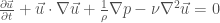
is the velocity vector, \vec{x} is position, \rho is density, p is pressure, and \nu is the kinematic viscosity. This equation can be made non-dimensional by the introduction of a characteristic velocity U, length L, and introducing the dynamic viscosity \eta=\nu/\rho. This gives the following dimensionless variables:

u^* = \frac{u}{U}

x^* = \frac{x}{L}

p^* = \frac{pL}{\eta U}

t^* = \frac{L}{U}

Substituting in these characteristic length scales and doing some algebra, one arrives at the simplified equations:

R\frac{\partial \vec{u^*}}{\partial t^*}+ R\vec{u^*}\cdot\nabla^*\vec{u^*} +\nabla^* p^*-(\nabla^*)^2\vec{u^*}=0

with only one dimensionless constant, the Reynold’s number, defined as:

R = \frac{UL\rho}{\eta} = \frac{UL}{\nu}

As explained in the paper, Reynold’s number is one of the essential constants describing a flow. High Reynold’s number leads to turbulent (chaotic) flow, while low Reynold’s number leads to laminar (smooth) flow. For extemely small Reynold’s number, Navier-Stokes simplifies to:

\nabla^* p^* = (\nabla^*)^2\vec{u^*}

which is also just called Stoke’s equation.

At the end of the paper, Purcell describes another dimensionless number which he calls S and in a footnote identifies as the Sherwood number. However, Ben Regner pointed out, that Purcell’s S would actually be called the Peclet number today.

Basics of Ecoli Chemotaxis

Chemotaxis and cellular sensing really deserves its own series of papers. But in the meantime, I recommend the following resources

Video Proof of Purcell’s Scallop Theorem

Reversible kicking does fine in water (high Reynold’s number)…

… but the same motion has issues in corn syrup (low Reynold’s number).

Here is a solution similar to what Ecoli and other bacteria employ.


Fundamental Questions

  • Purcell does an amazing job, so I have nothing to add.

Advanced Questions

  • What are some other strategies that are employed in biology to get around the issue of mobility at low Reynold’s number? Hint: I already linked to a video of one strategy. There are at least two other strategies, but to find these you will need to think about the assumptions leading to the basic Navier-Stokes equations.

Anomalous Diffusion

This is part of my “journal club for credit” series. You can see the other computational neuroscience papers in this post.

Unit: Diffusion

Organized by Ben Regner

  1. Standard Diffusion
  2. Anomalous Diffusion
  3. Life at Low Reynold’s Number

Papers

Other Useful References

What is anomalous diffusion?

If one measures the mean square displacement vs time, it can be parameterized as

< x^2> = t^\alpha

where \alpha=1 is Brownian (standard diffusion), 0<\alpha<1 is subdiffusive, 1<\alpha<2 is superdiffusive, and ballistic is \alpha=2. So the technical definition of anomalous diffusion is 0<\alpha<1 or 1<\alpha<2.

How to describe anomalous diffusion?

Currently, there is no “best” or “simple” description of anomalous diffusion in the general case. However, continuous-time random walks (CTRW) are one paradigm that I find helpful as a conceptual and simulation framework.

In the simplest discrete random walk (DRW), at every time step, a particle makes a jump of fixed size, the only question is the direction. The next generalization has the particle make a jump at every time step, but now it draws the jump size from a distribution.

The idea of a CTRW is that there is now a distribution both of the waiting time between jumps, and the jump size. If the waiting time follows the exponential distribution and the jump size follows the normal distribution, one ends up with the Wiener process aka standard diffusion and Brownian motion.

What causes anomalous diffusion?

Just as a reminder, there are three conditions that need to be satisfied for Brownian motion (standard diffusion):
1. Increments are independent
2. Increments are wide sense stationary. 1st moment and autocovariance don’t depend on time (this is weaker condition then complete stationarity)
3. Zero mean

The third condition is often ignored by examining the motion relative to the mean displacement (ie the actual displacement is not Brownian, but fluctuations in the displacement could be Brownian). So really, the first two are the more important conditions. Therefore, anomalous diffusion arises due to non-independent increments and/or correlations in time of the mean and/or standard deviation.

The CTRW allows one to think more precisely about different mechanisms that can give rise to anomalous diffusion. There is not one single way to get sub or super-diffusion in CTRW, since there are two, potentially dependent, distributions (waiting time and jump size). However, there are a few common situations that seem to arise often in biology and elsewhere (see Random walk models in biology, Box 2 for original idea). Subdiffusion in biology is often caused by longer waiting time distributions (compared to exponential), or molecular crowding, while superdiffusion in occurs when jump sizes are drawn from a Levy flight or other alpha stable distributions.

Examples

For further exploration of anomalous diffusion in biology, I recommend these papers

Advanced Questions

  • This is an interesting paper that introduces a renormalization group approach to classifying diffusion processes

Standard Diffusion

This is part of my “journal club for credit” series. You can see the other computational neuroscience papers in this post.

Unit: Diffusion

Organized by Ben Regner

  1. Standard Diffusion
  2. Anomalous Diffusion
  3. Life at Low Reynold’s Number

Papers

Brownian Motion. By Einstein in 1905.

Brownian Motion. By Langevin in 1908.

An Introduction to Fractional Diffusion. By Henry, Langlands, and Straka in 2010.

Other Useful References


What is diffusion?

Diffusion is the general process by which small particles move from regions of high concentration to low concentration. Check out the link to the Wikipedia articles above for some cool videos and animations. Diffusion is extremely ubiquitous and plays an essential role in biology. For example, oxygen diffuses from your lungs to unoxygenated blood, which then delivers it to the rest of your body where it diffuses out of your blood and into your cells. Additionally, signals between neurons are transmitted by several different diffusing molecules.

Mathematically, standard diffusion is described by two fundamental equations.

Fick’s First Law: Particles move from high-to-low concentration.

j=-D\frac{\partial n}{\partial x}

where n is the number of particles, x is the location of the particles, D is the diffusion constant, and  j is the flux of particles.

Fick’s Second Law: Conservation of particles combined with Fick’s First Law leads to the diffusion equation.

If particles cannot be created or destroyed, they follow a conservation law:

\frac{\partial n}{\partial t} = -\frac{\partial j}{\partial x}

Combining the conservation law with Fick’s First Law gives us the diffusion equation:

\frac{\partial n}{\partial t} = D \frac{\partial^2 n}{\partial x^2}

Brownian Motion

In 1827 Robert Brown looked at pollen in water under a microscope, see Wikipedia page for simulations of the observations. Much to his surprise, the pollen acts as if it alive! Brown verified that pollen is not alive and any small, inorganic particle followed similar motion. In 1905, during Einstein’s miracle year, he wrote a paper on an atomistic description that describes Brownian Motion. In 1908 Langevin used a different approach (that is “infinitely simpler” in his words) to describe Brownian motion. The general explanations are outlined below.

1. Einstein’s Derivation

Einstein’s goal was a probability based description of Brownian motion that connects to Fick’s law. Einstein makes several assumptions about the particles, including

In the end, Einstein finds a solution that is Gaussian, implying that the mean square displacement is linear in time for Brownian motion:

< x^2> = t

More generally, the mean square displacement could depend on some power of time, usually parameterized as

< x^2> = t^\alpha

where \alpha=1 is Brownian, 0<\alpha<1 is subdiffusive, 1<\alpha<2 is superdiffusive, and ballistic is \alpha=2. Note, one can get up to \alpha=3 in certain turbulent regimes.

2. Langevin’s Derivation
The Langevin approach is to start with a particle based description. The first assumption is the equipartition theorem to determine the kinetic energy (KE)
KE = \frac{k_B T}{2} = m (\frac{d^2 x}{dt^2})^2

Then, one looks at the actual forces on the particle:

KE = Stoke’s + stochastic variable
m (\frac{d^2 x}{dt^2})^2 = -6 \pi \eta r \frac{dx}{dt} + X
where X is a stochastic variable. It is assumed to be zero mean, unit variance, and no time correlations, aka white noise.

After multiplying both sides of the equation by x, doing some algebra, and then taking the average solution, one arrives at the same results as Einstein (after ignore a short time transient).


3. Random Walk Derivation.

There is a third way to derive Brownian motion that is layed out in the book chapter above. The idea is to look at a single particle and do a microscopic random walk. One can set up a recursive definition that defines a binomial probability solution. After a large number of steps, the central limit theorem applies and we end up with a Gaussian solution.

How do we get Brownian motion?

In general, there are three conditions that need to be satisfied for Brownian motion:
1. Increments are independent
2. Increments are wide sense stationary. 1st moment and autocovariance don’t depend on time (this is weaker condition then complete stationarity)
3. Zero mean

The third condition is often ignored by examining the motion relative to the mean displacement (ie the actual displacement is not Brownian, but fluctuations in the displacement could be Brownian). So really, the first two are the more important conditions.


Fundamental Questions

  • Einstein made three major assumptions in his derivation. 2/3 are often violated by biology, which assumption is relatively safe?
  • What biological processes do you think are actually diffusive vs sub/super-diffusive? Think about the 3 conditions for Brownian motion listed above. Note, this is a preview for the next post.

Advanced Questions

Deep Learning

This is part of my “journal club for credit” series. You can see the other computational neuroscience papers in this post.

Unit: Deep Learning

  1. Perceptron
  2. Energy Based Neural Networks
  3. Training Networks
  4. Deep Learning

Papers

Deep Learning. By LeCun, Bengio, and Hinton in 2015.

Deep learning in neural networks: An overview. By Schmidhuber in 2015.

Other Useful References


What is deep learning?

In previous weeks we have introduced perceptrons, multilayer perceptrons (MLP), Hopfield neural networks, and Boltzmann machines.

But what is deep learning? I think it is really two things:

  1. Successful training of multilayered neural networks perform better (higher classification accuracy, etc) and involve more layers than previous implementations
  2. Just a rebranding of neural networks

Here is my summary of the history of deep learning, see both reviews above for extended details. In 2006, Deep Belief Networks (DBN) were introduced in two papers (Reducing the Dimensionality of Data with Neural Networks and A Fast Learning Algorithm for Deep Belief Nets). The idea of a DBN is to train a series of restricted Boltzmann machines (RBM). The first RBM is trained and given the original data, produces an output of hidden layer activations. The second RBM uses the first RBM’s hidden layer activations as inputs, and trains on that “data”. This is continued to the desired depth. At this point, the DBN can be used for unsupervised learning, or one can use it as pretraining for a MLP which will utilize backpropagation for supervised learning.

So on the one hand, there were technical breakthroughs that enabled neural networks to utilize more layers than previous iterations and achieve state of the art performance. However, the actual component (RBMs and MLPs), have been around since the 1980s, so it would also be fair to deem deep learning as a rebranding of neural networks.

Therefore, neural network winter (mid 90s to mid 00s) officially ended in 2006. I propose calling 2006-2012 neural network spring. While interest in neural networks increased and new advances were made, the general machine learning community was not obsessed with deep learning. That changed in 2012 when the neural network summer began. This paper presented at NIPS revolutionized the computer vision community by cutting the error rate on Imagenet in half! The Imagenet challenge was viewed as a serious benchmark that all computer vision systems should address. By blowing previous results out of the water, the revolution was completed.

So for now, enjoy neural network summer, but always remember, winter is coming.

Fundamental Questions

  • When do extra layers help in a neural network? When do they hurt?
  • Why was pretraining originally needed, but is no longer used in practice? Check out these papers for details: Glorot and Saxe.
  • Learn about convolutional and recurrent neural networks. These are extremely popular right now!

Advanced Questions

  • Do research on unsupervised learning! It is definitely less popular today, but all the big-shots think is the longterm future of neural networks.

Training Networks

This is part of my “journal club for credit” series. You can see the other computational neuroscience papers in this post.

Unit: Deep Learning

  1. Perceptron
  2. Energy Based Neural Networks
  3. Training Networks
  4. Deep Learning

Papers

A Learning Algorithm for Boltzmann Machines. By Ackley, Hinton, and Sejnowski in 1985.

Learning representations by back-propagating errors. By Rumelhart, Hinton, and Williams in 1986.

Other Useful References


How do you actually train neural networks?

Hopefully the past few posts have piqued your interest in neural networks. Maybe you even want to unleash a neural network on some data. How do you actually train the neural network?

I’m actually going to keep this brief for two reasons. First, detailed derivations can already be found elsewhere (for Boltzmann see Appendix of the original paper as well as MacKay, for backpropagation see Nielsen). Second, I firmly believe that algorithms are best learned by actually stepping through the updates, so any explanation I attempt will not be sufficient for you to truly learn the algorithm. I will provide some general context as well as some questions you should be able to answer, but please go do it yourself!

There are three general classes of machine learning based on the information received:

  • Unsupervised – data only. Boltzmann machine.
  • Supervised – data with labels. MLP with backpropagation.
  • Reinforcement – data, actions, and scores associated with each action. Deserves its own detailed post, but check out papers by DeepMind for cool applications.

The Boltzmann machine learning rule is an example of maximum likelihood. In practice, the original learning rule is too computationally expensive, so a modified algorithm called contrastive divergence (or variants such as persistent contrastive divergence) is utilized instead. See the Hinton guide to RBMs for more details.

Backpropagation is a computationally-efficient writing of the chain rule from calculus, so besides the above paper which popularized it, there is actually a long history of this algorithm being discovered and rediscovered.

Fundamental Questions

  • What is maximum likelihood?
  • Why can one interpret the learning terms in the BM algorithm as “waking” and “sleeping”?
  • Why are BM hidden layers so important?
  • Why are restricted Boltzmann machines, RBMs, much easier to train?
  • Why is backpropagation more computationally efficient than the finite difference method?
  • Derive the 4 backpropagation equations!

Advanced Questions

  • Follow Hinton’s RBM guide and implement your own Boltzmann machine
  • Use Nielsen’s code to train your own MLP

Energy Based Neural Networks

This is part of my “journal club for credit” series. You can see the other computational neuroscience papers in this post.

Unit: Deep Learning

  1. Perceptron
  2. Energy Based Neural Networks
  3. Training Networks
  4. Deep Learning

Papers

Neural networks and physical systems with emergent collective computational abilities. By Hopfield in 1982.

A Learning Algorithm for Boltzmann Machines. By Ackley, Hinton, and Sejnowski in 1985. (Note: Only section 1 and 2 are covered here, rest of paper covered in next topic).

Other Useful References

  • Hopfield Network – Wikipedia and Scholarpedia
  • Boltzmann Machine – Wikipedia and Scholarpedia
  • MacKay, Ch 31 (optional intro to Ising model), Ch 42 (Hopfield), and Ch 43 (Boltzmann).
  • Amit – This provides a detailed, physics-based, analysis of the Hopfield model


Why should you care?

The Hopfield paper provides an explicit, decently biologically plausible, mechanism by which a system of (artificial) neurons can store memories. The central goal of the paper is to demonstrate a method for content-addressible memory. Standard computer memory is location-addressible (ie your computer looks to a specific place on your disk). The idea of content-addressible memory is that a partial (perhaps faulty) presentation of the memory should be sufficient to obtain the full memory. I love this quote:

An example asks you to recall ‘An American politician who was very intelligent and whose politician father did not like broccoli’. Many people think of president [George W.] Bush –even though one of the cues contains an error.

MacKay Ch 38, pg 469.

Hopfield Neural Network

So how does Hopfield actually store memories? The idea is that a system can be constructed such that the stable states of the system are the desired memories. I’m going to change notation from the original Hopfield paper so that it matches standard physics notation.

In the actual paper, Hopfield uses threshold neurons but all arguments can be easily extended to a tanh neuron. I will define a neuron’s state as S and neuron i (out of N total) is firing if S_i=1 and not firing if S_i = -1.

How does the system actually store memories? I will call the memories (p of them) that one wants to store as \xi^\mu where \mu=1\ldots p. The idea is to define the interactions between neurons as:

J_{ij} = \frac{1}{N}\sum_{\mu=1}^p \xi_i^\mu \xi_j^\mu

Why are memories actual stable? We can write the activation function of a neuron (also known as the local field in physics terms) as

a_i = \sum_{j\neq i} J_{ij} S_j

Now let’s check if a memory is stable (say memory 1) by examining the activation function of the first neuron.

a_1 = \sum_{j=2}^N J_{1j} \xi_j^1= \frac{1}{N} \sum_{j=2}^N \sum_{\mu=1}^p \xi_1^\mu \xi_j^\mu \xi_j^1

a_1 = \frac{1}{N} \sum_{j=2}^N \xi_1^1 +\frac{1}{N}\sum_{j=2}^N \sum_{\mu=2}^p \xi_1^\mu \xi_j^\mu \xi_j^1

a_1 = \frac{N-1}{N} \xi_1^1 +\frac{1}{N}\sum_{j=2}^N \sum_{\mu=2}^p \xi_1^\mu \xi_j^\mu \xi_j^1

The first term of the activation function is exactly what we need for the first neuron to be stable. The second term is noise, but how big is it? We need a couple more facts to figure it out. First, we can safely assume N\gg1. Second, we will assume that memories are not biased (equal numbers of neurons are on and off). Third, we will assume that we are storing random memories. Then using the central limit theorem, we get that on average, a_1 = \xi_1. (Advanced question: what is the standard deviation of the noise term? What does that imply about stability of memories?)

So this establishes that memories are stable. But how should we actually think about these memories? By examining the energy of the system, one can show that these memories are global minima and have basins of attraction. The energy is defined as

H = -\frac{1}{2} \sum_{ij} S_i J_{ij} S_j

where we have defined the self-interactions to be zero (J_{ii}=0). Using similar arguments as above, one can show that on average each memory has an energy of -\frac{N}{2} and that a flipping a single spin leads to higher energy. (Fundamental question: prove these statements!)

Therefore, using the prescription outlined in the Hopfield paper, one can take a set of memories, \xi, and create a dynamical system with these memories as global minima.


Boltzmann Machine

Hopfield networks are great if you already know the states of the desired memories. But what if you are only given data? How would you actually train a neural network to store the data?

The next journal club will get to actual training, but it is convenient to introduce at this time a Boltzmann Machine (BM). This is an extension of Hopfield networks that can actually learn to store data. In the most general Boltzmann machine, neurons are divided into visible (actually interact with the data) and hidden (only see data through interactions with visible neurons). This leads to an energy function of:

H = -\frac{1}{2} \sum_{ij}v_i J_{ij} v_j- \sum_{ij}v_i w_{ij} h_j-\frac{1}{2} \sum_{ij}h_i K_{ij} h_j

where v are visible neurons and h are hidden neurons (if present, not a requirement). There are three different types of interactions, those amongst visible neurons only (J), those amongst hidden neurons only (K), and those between visible and hidden neurons (w).

As will be explained in the next journal club, the full Boltzmann machine takes a long time to train. So instead, it is common to use a Restricted Boltzmann Machine (RBM) which has no self interactions amongst layers:

H = - \sum_{ij}v_i w_{ij} h_j


Fundamental Questions

  • Why is content-addressible memory considered associative, software and hardware fault tolerant, and distributed? Why is this closer to biology than location-addressible memory?
  • Why is the Hopfield storage prescription Hebbian?
  • Do the calculation to show that the memories are global minima.
  • Hopfield says “In many physical systems, the nature of the emergent collective properties are insensitive to the details inserted in the model.” What are some assumptions that Hopfield relaxes in the simulations?
  • Next time we will see that RBMs are easier to train to BM. Can you see why?

Advanced Questions

  • For the activation function argument, what is the standard deviation of the noise term? What does that imply about stability of memories?
  • What happens to the capacity if the memories are not equally \pm 1 and/or correlated with each other?

Perceptron

This is part of my “journal club for credit” series. You can see the other computational neuroscience papers in this post.

Unit: Deep Learning

  1. Perceptron
  2. Energy Based Neural Networks
  3. Training Networks
  4. Deep Learning

Paper

The Perceptron: A Probabilistic Model for Information Storage and Organization in the Brain by Rosenblatt in 1958

Other Useful References

Motivation for Perceptron

I’ll let Rosenblatt introduce the important questions leading to the perceptron himself by quoting his first paragraph:

If we are eventually to understand the capability of higher organisms for perceptual recognition, generalization, recall, and thinking, we must first have answers to three fundamental questions:

  1. How is information about the physical world sensed, or detected, by biological system?
  2. In what form is information stored, or remembered?
  3. How does information in storage, or in memory, influence recognition and behavior?

The perceptron is a first attempt to answer second and third questions. In the years leading up to the perceptron, there were two dominate themes of theoretical research on the brain. One focused on the general computational properties of the brain (McCollough and Pitts 1943) and showed that simple binary neurons could form a computer (ie they can compute any possible function). Another theme focused on abstracting away the details of experiments to get at general principles that relate to computation in the brain (Hebb 1949 and his synapse learning rules).

The perceptron opened up a third avenue of theoretical research. The central goal is to devise neuron-inspired algorithms that learn from real data and can be used to make a decision.

What is a Perceptron?

Basics

I find the math in the original perceptron paper pretty confusing. This is partly due to a generational difference in terminology, and partly due to poor explanations in the paper. This is definitely a paper that benefited from the passage of time and future synthesis into a more concise topic. Therefore, I recommend focusing attention on the introduction and conclusion, while below I’ll introduce the modern notation of the perceptron (see MacKay Ch 39/40 for similar details).

Perceptron

The perceptron consists of a set of inputs, x, that are fed into the perceptron, with each input receiving its own weight, w. The activity of the percepton is given by a = wx

Note that the perceptron can have a bias that is independent of inputs. However, we don’t need to write this out separately and can instead include an input that is always set to 1, independently of the data.

This activity is then evaluated by the activation function, f(a), to determine the output, y. There are lots of different possible activation rules with some popular ones including

  • Linear:

y(a) = a

  • Rectified Linear:

\begin{aligned} y &= 0 \quad\text{if}\quad a \leq 0 \\ y&= a\quad\text{if}\quad a>0 \end{aligned}

  • Sigmoid:

y(a) = \frac{1}{1+\exp{(-a)}}

  • Threshold:

\begin{aligned} y &= 0 \quad\text{if}\quad a \leq 0 \\ y&= 1\quad\text{if}\quad a>0 \end{aligned}


The end result is that we can take the output of a perceptron and use this output to make a decision. The sigmoid and threshold activation functions return an answer between 0 and 1 and hence have a natural interpretation as a probability. From now on, we will work with sigmoid activation functions.

Training

Now that the basics of a perceptron have been introduced, how do we actually train it? In other words, if I gave you a set of data, X, where each entry x_n is N dimensional, how would I evaluate perceptron’s handling of the data? For now, we will focus on using the perceptron as a binary classifier (only need to decide between two groups: 0 and 1). Since we are using sigmoid activation functions, we can interpret the output as the probability that the data is in group 1.

The standard way to train a binary classier is to have a training set which consists of pairs of data, x_n, and correct labels, t_n. Then training proceeds by seeing if the output label of a perceptron matches the correct label. If everything is correct, perfect! If not, we need to do something with that error.

For a sigmoid activation, the commonly used error function is the cross-entropy:

\mathcal{E} = - \sum_n \left[ t_n \ln y_n + \left(1-t_n \right) \ln \left(1-y_n \right) \right]

The output y is a function of the weights w. We can then take the derivate of the error with respect to the weights, which in the case of the sigmoid activation and cross-entropy error is simply \delta \mathcal{E}_n = -\left(t_n - y_n\right) x_n.

The simplest possible update algorithm is to perform gradient descent on the weights and define \Delta w_n =\delta \mathcal{E}_n. This is a greedy algorithm (always improves current error, longterm consequences be damned!). Gradient descent comes in several closely related varieties: online, batch, and mini-batch. Let’s start with the mini-batch. First the data is divided up into small random sets (say 10 data points each). Then we loop through the mini-batches, and for each one we calculate the output and error and update the weights. Online learning is when the mini-batches each contain exactly 1 data point, while batch learning is when the mini-batch is the whole dataset. The current standard is to use a mini-batch of between 10 to 100 which is a compromise between speed (batches are faster) and accuracy (online finds better solutions).

Putting it all together, the training algorithm is as follows

  1. Calculate the activation function and output with respect to a mini-batch of data
  2. Calculate the errors of the output
  3. Update the weights


And now you’ve got all the basics of a perceptron down! On to the more difficult questions…

Fundamental Questions

  • What are similarities and differences between a perceptron and a neuron? Do different activation functions lead to distinct interpretations?
  • What is connectivisim? How does this relate to the perceptron? How does this contrast with computers?
  • What class of learning algorithm is the perceptron? Possible answers: unsupervised, supervised, or reinforcement learning
  • What type of functions can a perceptron compute? Compare the standard OR gate vs the exclusive OR (XOR) gate for a perceptron with 2 weights.
  • Does the perceptron return a unique answer? Does the perceptron return the “best” answer (you need to define “best”)? Check out Support Vector Machines for one answer to the “best”.
  • Under what conditions can the perceptron generalize to data it has never seen before? Look into Rosenblatt’s “differentiated environment”.

Additional Questions

  • There are other possibilities for the error functions. Why is the cross-entropy a wise choice for the sigmoid activation?
  • The weight updates can be multiplied by a “learning rate” that controls the size of updates, while I implicitly assumed a learning rate of 1. How would you actually determine a sensible learning rate?
  • The standard learning algorithm puts no constraints on the possible weights. What are some possible problems with unconstrained weights? Can you think of a possible solution? How does this change the generalization properties of a perceptron?
  • Threshold activation functions produce simpler output (only two possible values) than sigmoid activation functions. Despite this simpler output, threshold activation functions are more difficult to train. Can you figure out why?
  • What is the information storage capacity of a perceptron? The exact answer is difficult, but you can get the right order of magnitude in the limit of large number of data points and large number of weights.


JC: Computational Neuroscience

This is part of the “journal club for credit” series. Below are the included units and details for each week.

Unit: Deep Learning

  1. Perceptron
  2. Energy Based Neural Networks
  3. Training Networks
  4. Deep Learning

Unit: Diffusion

Organized by Ben Regner

  1. Standard Diffusion
  2. Anomalous Diffusion
  3. Life at Low Reynold’s Number