Life at Low Reynolds Number

This is part of my “journal club for credit” series. You can see the other computational neuroscience papers in this post.

Unit: Diffusion

Organized by Ben Regner

  1. Standard Diffusion
  2. Anomalous Diffusion
  3. Life at Low Reynold’s Number

Papers

Life at Low Reynold’s Number. By Purcell in 1977.

Other Useful References

Introduction

This is one of my favorite papers. The presentation style is extremely fun and readable without sacrificing any scientific integrity. I think it serves as a great introduction to fluid mechanics at low Reynold’s number. I don’t have too many comments since I think the paper explains it the best, but I will provide a few supplementary details for a more in depth exploration of the ideas from the paper.

And just to get you excited about fluid dynamics, I present an example of laminar flow:

Basics of Fluid Mechanics

The fundamental equation of fluid mechanics is Navier-Stokes. The relevant version for this paper is the incompressible flow equations with pressure but no other external fields:
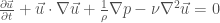
\frac{\partial \vec{u}}{\partial t}+ \vec{u}\cdot\nabla\vec{u} +\frac{1}{\rho}\nabla p -\nu\nabla^2\vec{u}=0

where \vec{u} is the velocity vector, \vec{x} is position, \rho is density, p is pressure, and \nu is the kinematic viscosity. This equation can be made non-dimensional by the introduction of a characteristic velocity U, length L, and introducing the dynamic viscosity \eta=\nu/\rho. This gives the following dimensionless variables:

u^* = \frac{u}{U}

x^* = \frac{x}{L}

p^* = \frac{pL}{\eta U}

t^* = \frac{L}{U}

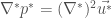
Substituting in these characteristic length scales and doing some algebra, one arrives at the simplified equations:

R\frac{\partial \vec{u^*}}{\partial t^*}+ R\vec{u^*}\cdot\nabla^*\vec{u^*} +\nabla^* p^*-(\nabla^*)^2\vec{u^*}=0

with only one dimensionless constant, the Reynold’s number, defined as:

R = \frac{UL\rho}{\eta} = \frac{UL}{\nu}

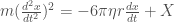
As explained in the paper, Reynold’s number is one of the essential constants describing a flow. High Reynold’s number leads to turbulent (chaotic) flow, while low Reynold’s number leads to laminar (smooth) flow. For extemely small Reynold’s number, Navier-Stokes simplifies to:

\nabla^* p^* = (\nabla^*)^2\vec{u^*}

which is also just called Stoke’s equation.

At the end of the paper, Purcell describes another dimensionless number which he calls S and in a footnote identifies as the Sherwood number. However, Ben Regner pointed out, that Purcell’s S would actually be called the Peclet number today.

Basics of Ecoli Chemotaxis

Chemotaxis and cellular sensing really deserves its own series of papers. But in the meantime, I recommend the following resources

Video Proof of Purcell’s Scallop Theorem

Reversible kicking does fine in water (high Reynold’s number)…

… but the same motion has issues in corn syrup (low Reynold’s number).

Here is a solution similar to what Ecoli and other bacteria employ.


Fundamental Questions

  • Purcell does an amazing job, so I have nothing to add.

Advanced Questions

  • What are some other strategies that are employed in biology to get around the issue of mobility at low Reynold’s number? Hint: I already linked to a video of one strategy. There are at least two other strategies, but to find these you will need to think about the assumptions leading to the basic Navier-Stokes equations.
Advertisement

Anomalous Diffusion

This is part of my “journal club for credit” series. You can see the other computational neuroscience papers in this post.

Unit: Diffusion

Organized by Ben Regner

  1. Standard Diffusion
  2. Anomalous Diffusion
  3. Life at Low Reynold’s Number

Papers

Other Useful References

What is anomalous diffusion?

If one measures the mean square displacement vs time, it can be parameterized as

< x^2> = t^\alpha

where \alpha=1 is Brownian (standard diffusion), 0<\alpha<1 is subdiffusive, 1<\alpha<2 is superdiffusive, and ballistic is \alpha=2. So the technical definition of anomalous diffusion is 0<\alpha<1 or 1<\alpha<2.

How to describe anomalous diffusion?

Currently, there is no “best” or “simple” description of anomalous diffusion in the general case. However, continuous-time random walks (CTRW) are one paradigm that I find helpful as a conceptual and simulation framework.

In the simplest discrete random walk (DRW), at every time step, a particle makes a jump of fixed size, the only question is the direction. The next generalization has the particle make a jump at every time step, but now it draws the jump size from a distribution.

The idea of a CTRW is that there is now a distribution both of the waiting time between jumps, and the jump size. If the waiting time follows the exponential distribution and the jump size follows the normal distribution, one ends up with the Wiener process aka standard diffusion and Brownian motion.

What causes anomalous diffusion?

Just as a reminder, there are three conditions that need to be satisfied for Brownian motion (standard diffusion):
1. Increments are independent
2. Increments are wide sense stationary. 1st moment and autocovariance don’t depend on time (this is weaker condition then complete stationarity)
3. Zero mean

The third condition is often ignored by examining the motion relative to the mean displacement (ie the actual displacement is not Brownian, but fluctuations in the displacement could be Brownian). So really, the first two are the more important conditions. Therefore, anomalous diffusion arises due to non-independent increments and/or correlations in time of the mean and/or standard deviation.

The CTRW allows one to think more precisely about different mechanisms that can give rise to anomalous diffusion. There is not one single way to get sub or super-diffusion in CTRW, since there are two, potentially dependent, distributions (waiting time and jump size). However, there are a few common situations that seem to arise often in biology and elsewhere (see Random walk models in biology, Box 2 for original idea). Subdiffusion in biology is often caused by longer waiting time distributions (compared to exponential), or molecular crowding, while superdiffusion in occurs when jump sizes are drawn from a Levy flight or other alpha stable distributions.

Examples

For further exploration of anomalous diffusion in biology, I recommend these papers

Advanced Questions

  • This is an interesting paper that introduces a renormalization group approach to classifying diffusion processes

Standard Diffusion

This is part of my “journal club for credit” series. You can see the other computational neuroscience papers in this post.

Unit: Diffusion

Organized by Ben Regner

  1. Standard Diffusion
  2. Anomalous Diffusion
  3. Life at Low Reynold’s Number

Papers

Brownian Motion. By Einstein in 1905.

Brownian Motion. By Langevin in 1908.

An Introduction to Fractional Diffusion. By Henry, Langlands, and Straka in 2010.

Other Useful References


What is diffusion?

Diffusion is the general process by which small particles move from regions of high concentration to low concentration. Check out the link to the Wikipedia articles above for some cool videos and animations. Diffusion is extremely ubiquitous and plays an essential role in biology. For example, oxygen diffuses from your lungs to unoxygenated blood, which then delivers it to the rest of your body where it diffuses out of your blood and into your cells. Additionally, signals between neurons are transmitted by several different diffusing molecules.

Mathematically, standard diffusion is described by two fundamental equations.

Fick’s First Law: Particles move from high-to-low concentration.

j=-D\frac{\partial n}{\partial x}

where n is the number of particles, x is the location of the particles, D is the diffusion constant, and  j is the flux of particles.

Fick’s Second Law: Conservation of particles combined with Fick’s First Law leads to the diffusion equation.

If particles cannot be created or destroyed, they follow a conservation law:

\frac{\partial n}{\partial t} = -\frac{\partial j}{\partial x}

Combining the conservation law with Fick’s First Law gives us the diffusion equation:

\frac{\partial n}{\partial t} = D \frac{\partial^2 n}{\partial x^2}

Brownian Motion

In 1827 Robert Brown looked at pollen in water under a microscope, see Wikipedia page for simulations of the observations. Much to his surprise, the pollen acts as if it alive! Brown verified that pollen is not alive and any small, inorganic particle followed similar motion. In 1905, during Einstein’s miracle year, he wrote a paper on an atomistic description that describes Brownian Motion. In 1908 Langevin used a different approach (that is “infinitely simpler” in his words) to describe Brownian motion. The general explanations are outlined below.

1. Einstein’s Derivation

Einstein’s goal was a probability based description of Brownian motion that connects to Fick’s law. Einstein makes several assumptions about the particles, including

In the end, Einstein finds a solution that is Gaussian, implying that the mean square displacement is linear in time for Brownian motion:

< x^2> = t

More generally, the mean square displacement could depend on some power of time, usually parameterized as

< x^2> = t^\alpha

where \alpha=1 is Brownian, 0<\alpha<1 is subdiffusive, 1<\alpha<2 is superdiffusive, and ballistic is \alpha=2. Note, one can get up to \alpha=3 in certain turbulent regimes.

2. Langevin’s Derivation
The Langevin approach is to start with a particle based description. The first assumption is the equipartition theorem to determine the kinetic energy (KE)
KE = \frac{k_B T}{2} = m (\frac{d^2 x}{dt^2})^2

Then, one looks at the actual forces on the particle:

KE = Stoke’s + stochastic variable
m (\frac{d^2 x}{dt^2})^2 = -6 \pi \eta r \frac{dx}{dt} + X
where X is a stochastic variable. It is assumed to be zero mean, unit variance, and no time correlations, aka white noise.

After multiplying both sides of the equation by x, doing some algebra, and then taking the average solution, one arrives at the same results as Einstein (after ignore a short time transient).


3. Random Walk Derivation.

There is a third way to derive Brownian motion that is layed out in the book chapter above. The idea is to look at a single particle and do a microscopic random walk. One can set up a recursive definition that defines a binomial probability solution. After a large number of steps, the central limit theorem applies and we end up with a Gaussian solution.

How do we get Brownian motion?

In general, there are three conditions that need to be satisfied for Brownian motion:
1. Increments are independent
2. Increments are wide sense stationary. 1st moment and autocovariance don’t depend on time (this is weaker condition then complete stationarity)
3. Zero mean

The third condition is often ignored by examining the motion relative to the mean displacement (ie the actual displacement is not Brownian, but fluctuations in the displacement could be Brownian). So really, the first two are the more important conditions.


Fundamental Questions

  • Einstein made three major assumptions in his derivation. 2/3 are often violated by biology, which assumption is relatively safe?
  • What biological processes do you think are actually diffusive vs sub/super-diffusive? Think about the 3 conditions for Brownian motion listed above. Note, this is a preview for the next post.

Advanced Questions

Webmaster Buddy

Feel free to leave comments on posts. In order to stop spam, if you are a first time commenter, your comment will be held and must be approved by the webmaster Buddy:

Buddy_computer

Whether your comment is deemed spam will be arbitrarily decided by the whims of Buddy. He can be bribed with treats such as peanut butter and Cesar’s. Don’t expect a prompt response, since Buddy’s usual state is this:

Buddy_sleep

Deep Learning

This is part of my “journal club for credit” series. You can see the other computational neuroscience papers in this post.

Unit: Deep Learning

  1. Perceptron
  2. Energy Based Neural Networks
  3. Training Networks
  4. Deep Learning

Papers

Deep Learning. By LeCun, Bengio, and Hinton in 2015.

Deep learning in neural networks: An overview. By Schmidhuber in 2015.

Other Useful References


What is deep learning?

In previous weeks we have introduced perceptrons, multilayer perceptrons (MLP), Hopfield neural networks, and Boltzmann machines.

But what is deep learning? I think it is really two things:

  1. Successful training of multilayered neural networks perform better (higher classification accuracy, etc) and involve more layers than previous implementations
  2. Just a rebranding of neural networks

Here is my summary of the history of deep learning, see both reviews above for extended details. In 2006, Deep Belief Networks (DBN) were introduced in two papers (Reducing the Dimensionality of Data with Neural Networks and A Fast Learning Algorithm for Deep Belief Nets). The idea of a DBN is to train a series of restricted Boltzmann machines (RBM). The first RBM is trained and given the original data, produces an output of hidden layer activations. The second RBM uses the first RBM’s hidden layer activations as inputs, and trains on that “data”. This is continued to the desired depth. At this point, the DBN can be used for unsupervised learning, or one can use it as pretraining for a MLP which will utilize backpropagation for supervised learning.

So on the one hand, there were technical breakthroughs that enabled neural networks to utilize more layers than previous iterations and achieve state of the art performance. However, the actual component (RBMs and MLPs), have been around since the 1980s, so it would also be fair to deem deep learning as a rebranding of neural networks.

Therefore, neural network winter (mid 90s to mid 00s) officially ended in 2006. I propose calling 2006-2012 neural network spring. While interest in neural networks increased and new advances were made, the general machine learning community was not obsessed with deep learning. That changed in 2012 when the neural network summer began. This paper presented at NIPS revolutionized the computer vision community by cutting the error rate on Imagenet in half! The Imagenet challenge was viewed as a serious benchmark that all computer vision systems should address. By blowing previous results out of the water, the revolution was completed.

So for now, enjoy neural network summer, but always remember, winter is coming.

Fundamental Questions

  • When do extra layers help in a neural network? When do they hurt?
  • Why was pretraining originally needed, but is no longer used in practice? Check out these papers for details: Glorot and Saxe.
  • Learn about convolutional and recurrent neural networks. These are extremely popular right now!

Advanced Questions

  • Do research on unsupervised learning! It is definitely less popular today, but all the big-shots think is the longterm future of neural networks.